Lecture 13 – Working with data using R / tidyverse
Arvind R. Subramaniam
Assistant Member
Basic Sciences Division and Computational Biology Program
Fred Hutchinson Cancer Research Center
Tidyverse Functions for Working with Tabular Data
| Import/Export | Visualize | Transform |
|---|---|---|
read_tsv |
geom_point |
select |
write_tsv |
geom_line |
filter |
facet_grid |
arrange |
|
mutate |
||
join |
||
group_by |
||
summarize |
Read tabular data into a DataFrame (tibble)
library(tidyverse)

data <- read_tsv("data/example_dataset_1.tsv")
print(data, n = 5)
# A tibble: 16 x 7
  strain  mean_yfp mean_rfp mean_ratio se_ratio insert_sequence kozak_region
  <chr>      <dbl>    <dbl>      <dbl>    <dbl> <chr>           <chr>
1 schp688     1748    20754      0.755    0.066 10×AGA          A
2 schp684     3294    20585      1.44     0.021 10×AGA          B
3 schp690     3535    20593      1.54     0.018 10×AGA          C
4 schp687     4658    20860      2.00     0.021 10×AGA          D
5 schp686     5000    21171      2.12     0.023 10×AGA          E
# … with 11 more rows
Use the pipe %>% operator to chain commands
data %>%
  print(n = 5)
# A tibble: 16 x 7
  strain  mean_yfp mean_rfp mean_ratio se_ratio insert_sequence kozak_region
  <chr>      <dbl>    <dbl>      <dbl>    <dbl> <chr>           <chr>
1 schp688     1748    20754      0.755    0.066 10×AGA          A
2 schp684     3294    20585      1.44     0.021 10×AGA          B
3 schp690     3535    20593      1.54     0.018 10×AGA          C
4 schp687     4658    20860      2.00     0.021 10×AGA          D
5 schp686     5000    21171      2.12     0.023 10×AGA          E
# … with 11 more rows
All these commands produce the same output.
print(data, n= 5)
data %>%
    print(., n = 5)
data %>% print(n = 5)
Simple Data Manipulations – select columns
data %>%
  print(n = 2)
# A tibble: 16 x 7
  strain  mean_yfp mean_rfp mean_ratio se_ratio insert_sequence kozak_region
  <chr>      <dbl>    <dbl>      <dbl>    <dbl> <chr>           <chr>
1 schp688     1748    20754      0.755    0.066 10×AGA          A
2 schp684     3294    20585      1.44     0.021 10×AGA          B
# … with 14 more rows
data %>%
  select(strain, mean_ratio, insert_sequence, kozak_region) %>%
  print(n = 2)
# A tibble: 16 x 4
  strain  mean_ratio insert_sequence kozak_region
  <chr>        <dbl> <chr>           <chr>
1 schp688      0.755 10×AGA          A
2 schp684      1.44  10×AGA          B
# … with 14 more rows
Simple Data Manipulations – filter rows
data %>%
  filter(kozak_region == "A")
# A tibble: 2 x 7
  strain  mean_yfp mean_rfp mean_ratio se_ratio insert_sequence kozak_region
  <chr>      <dbl>    <dbl>      <dbl>    <dbl> <chr>           <chr>
1 schp688     1748    20754      0.755    0.066 10×AGA          A
2 schp679     2528    19906      1.15     0.056 10×AAG          A
data %>%
  filter(kozak_region == "A", insert_sequence == "10×AGA")
# A tibble: 1 x 7
  strain  mean_yfp mean_rfp mean_ratio se_ratio insert_sequence kozak_region
  <chr>      <dbl>    <dbl>      <dbl>    <dbl> <chr>           <chr>
1 schp688     1748    20754      0.755    0.066 10×AGA          A
data %>%
  filter(kozak_region == "A") %>%
  filter(insert_sequence == "10×AGA")
# A tibble: 1 x 7
  strain  mean_yfp mean_rfp mean_ratio se_ratio insert_sequence kozak_region
  <chr>      <dbl>    <dbl>      <dbl>    <dbl> <chr>           <chr>
1 schp688     1748    20754      0.755    0.066 10×AGA          A
Simple Data Manipulations – arrange rows
data %>%
  arrange(mean_ratio)
# A tibble: 16 x 7
   strain  mean_yfp mean_rfp mean_ratio se_ratio insert_sequence kozak_region
   <chr>      <dbl>    <dbl>      <dbl>    <dbl> <chr>           <chr>
 1 schp680     1117    19377      0.519    0.01  10×AAG          H
 2 schp674     1270    20316      0.561    0.004 10×AAG          G
 3 schp688     1748    20754      0.755    0.066 10×AGA          A
 4 schp679     2528    19906      1.15     0.056 10×AAG          A
 5 schp676     2657    20223      1.18     0.048 10×AAG          F
 6 schp684     3294    20585      1.44     0.021 10×AGA          B
 7 schp690     3535    20593      1.54     0.018 10×AGA          C
 8 schp675     3687    20438      1.62     0.036 10×AAG          B
 9 schp681     3705    20227      1.64     0.021 10×AAG          C
10 schp677     3967    20604      1.73     0.03  10×AAG          E
11 schp678     4378    20630      1.91     0.01  10×AAG          D
12 schp687     4658    20860      2.00     0.021 10×AGA          D
13 schp686     5000    21171      2.12     0.023 10×AGA          E
14 schp685     7379    22956      2.89     0.05  10×AGA          F
15 schp689     8693    22649      3.42     0.125 10×AGA          H
16 schp683     9365    23866      3.52     0.11  10×AGA          G
Use mutate to create new columns
data <- read_tsv("data/example_dataset_2.tsv") %>%
    print()
# A tibble: 16 x 3
   strain  mean_yfp mean_rfp
   <chr>      <int>    <int>
 1 schp688     1748    20754
 2 schp684     3294    20585
 3 schp690     3535    20593
 4 schp687     4658    20860
 5 schp686     5000    21171
 6 schp685     7379    22956
 7 schp683     9365    23866
 8 schp689     8693    22649
 9 schp679     2528    19906
10 schp675     3687    20438
11 schp681     3705    20227
12 schp678     4378    20630
13 schp677     3967    20604
14 schp676     2657    20223
15 schp674     1270    20316
16 schp680     1117    19377
Use mutate to create new columns
data <- data %>%
  mutate(mean_ratio = mean_yfp / mean_rfp) %>%
  print()
# A tibble: 16 x 4
   strain  mean_yfp mean_rfp mean_ratio
   <chr>      <dbl>    <dbl>      <dbl>
 1 schp688     1748    20754     0.0842
 2 schp684     3294    20585     0.160
 3 schp690     3535    20593     0.172
 4 schp687     4658    20860     0.223
 5 schp686     5000    21171     0.236
 6 schp685     7379    22956     0.321
 7 schp683     9365    23866     0.392
 8 schp689     8693    22649     0.384
 9 schp679     2528    19906     0.127
10 schp675     3687    20438     0.180
11 schp681     3705    20227     0.183
12 schp678     4378    20630     0.212
13 schp677     3967    20604     0.193
14 schp676     2657    20223     0.131
15 schp674     1270    20316     0.0625
16 schp680     1117    19377     0.0576
Use mutate to modify existing columns
data %>%
  mutate(mean_ratio = round(mean_ratio, 2)) %>%
  print()
# A tibble: 16 x 4
   strain  mean_yfp mean_rfp mean_ratio
   <chr>      <dbl>    <dbl>      <dbl>
 1 schp688     1748    20754       0.08
 2 schp684     3294    20585       0.16
 3 schp690     3535    20593       0.17
 4 schp687     4658    20860       0.22
 5 schp686     5000    21171       0.24
 6 schp685     7379    22956       0.32
 7 schp683     9365    23866       0.39
 8 schp689     8693    22649       0.38
 9 schp679     2528    19906       0.13
10 schp675     3687    20438       0.18
11 schp681     3705    20227       0.18
12 schp678     4378    20630       0.21
13 schp677     3967    20604       0.19
14 schp676     2657    20223       0.13
15 schp674     1270    20316       0.06
16 schp680     1117    19377       0.06
Use TYPE_join to join two data frames
annotations <- read_tsv("data/example_dataset_3.tsv") %>%
  print()
# A tibble: 17 x 3
   strain  insert_sequence kozak_region
   <chr>   <chr>           <chr>
 1 schp674 10×AAG          G
 2 schp675 10×AAG          B
 3 schp676 10×AAG          F
 4 schp677 10×AAG          E
 5 schp678 10×AAG          D
 6 schp679 10×AAG          A
 7 schp680 10×AAG          H
 8 schp681 10×AAG          C
 9 schp683 10×AGA          G
10 schp684 10×AGA          B
11 schp685 10×AGA          F
12 schp686 10×AGA          E
13 schp687 10×AGA          D
14 schp688 10×AGA          A
15 schp689 10×AGA          H
16 schp690 10×AGA          C
17 control <NA>            <NA>
inner_join keeps common rows
data %>%
  inner_join(annotations, by = "strain") %>%
  print()
# A tibble: 16 x 6
   strain  mean_yfp mean_rfp mean_ratio insert_sequence kozak_region
   <chr>      <dbl>    <dbl>      <dbl> <chr>           <chr>
 1 schp688     1748    20754     0.0842 10×AGA          A
 2 schp684     3294    20585     0.160  10×AGA          B
 3 schp690     3535    20593     0.172  10×AGA          C
 4 schp687     4658    20860     0.223  10×AGA          D
 5 schp686     5000    21171     0.236  10×AGA          E
 6 schp685     7379    22956     0.321  10×AGA          F
 7 schp683     9365    23866     0.392  10×AGA          G
 8 schp689     8693    22649     0.384  10×AGA          H
 9 schp679     2528    19906     0.127  10×AAG          A
10 schp675     3687    20438     0.180  10×AAG          B
11 schp681     3705    20227     0.183  10×AAG          C
12 schp678     4378    20630     0.212  10×AAG          D
13 schp677     3967    20604     0.193  10×AAG          E
14 schp676     2657    20223     0.131  10×AAG          F
15 schp674     1270    20316     0.0625 10×AAG          G
16 schp680     1117    19377     0.0576 10×AAG          H
left_join keeps all rows in left data frame
data %>%
  left_join(annotations, by = "strain") %>%
  print()
# A tibble: 16 x 6
   strain  mean_yfp mean_rfp mean_ratio insert_sequence kozak_region
   <chr>      <dbl>    <dbl>      <dbl> <chr>           <chr>
 1 schp688     1748    20754     0.0842 10×AGA          A
 2 schp684     3294    20585     0.160  10×AGA          B
 3 schp690     3535    20593     0.172  10×AGA          C
 4 schp687     4658    20860     0.223  10×AGA          D
 5 schp686     5000    21171     0.236  10×AGA          E
 6 schp685     7379    22956     0.321  10×AGA          F
 7 schp683     9365    23866     0.392  10×AGA          G
 8 schp689     8693    22649     0.384  10×AGA          H
 9 schp679     2528    19906     0.127  10×AAG          A
10 schp675     3687    20438     0.180  10×AAG          B
11 schp681     3705    20227     0.183  10×AAG          C
12 schp678     4378    20630     0.212  10×AAG          D
13 schp677     3967    20604     0.193  10×AAG          E
14 schp676     2657    20223     0.131  10×AAG          F
15 schp674     1270    20316     0.0625 10×AAG          G
16 schp680     1117    19377     0.0576 10×AAG          H
right_join keeps all rows in right data frame
data %>%
  right_join(annotations, by = "strain") %>%
  print()
# A tibble: 17 x 6
   strain  mean_yfp mean_rfp mean_ratio insert_sequence kozak_region
   <chr>      <dbl>    <dbl>      <dbl> <chr>           <chr>
 1 schp688     1748    20754     0.0842 10×AGA          A
 2 schp684     3294    20585     0.160  10×AGA          B
 3 schp690     3535    20593     0.172  10×AGA          C
 4 schp687     4658    20860     0.223  10×AGA          D
 5 schp686     5000    21171     0.236  10×AGA          E
 6 schp685     7379    22956     0.321  10×AGA          F
 7 schp683     9365    23866     0.392  10×AGA          G
 8 schp689     8693    22649     0.384  10×AGA          H
 9 schp679     2528    19906     0.127  10×AAG          A
10 schp675     3687    20438     0.180  10×AAG          B
11 schp681     3705    20227     0.183  10×AAG          C
12 schp678     4378    20630     0.212  10×AAG          D
13 schp677     3967    20604     0.193  10×AAG          E
14 schp676     2657    20223     0.131  10×AAG          F
15 schp674     1270    20316     0.0625 10×AAG          G
16 schp680     1117    19377     0.0576 10×AAG          H
17 control       NA       NA    NA      <NA>            <NA>
Use summarize to calculate stats across rows
data %>%
  summarize(max_yfp = max(mean_yfp),
            max_rfp = max(mean_rfp)) %>%
  print()
# A tibble: 1 x 2
  max_yfp max_rfp
    <dbl>   <dbl>
1    9365   23866
Use summarize to calculate stats across rows
data %>%
  summarize(max_yfp = max(mean_yfp),
            max_rfp = max(mean_rfp)) %>%
  print()
# A tibble: 1 x 2
  max_yfp max_rfp
    <dbl>   <dbl>
1    9365   23866
Other examples of summary functions:
min() |
mean() |
sd() |
first() |
n() |
Use group_by to group subsets of rows
data <- read_tsv("data/example_dataset_4.tsv") %>%
  print(n = 10)
# A tibble: 74 x 4
   strain    yfp   rfp replicate
   <chr>   <int> <int>     <int>
 1 schp690  3640 20944         1
 2 schp690  3502 20881         2
 3 schp690  3569 20063         3
 4 schp690  3475 20773         4
 5 schp690  3487 20307         5
 6 schp689  9790 24399         1
 7 schp689  9821 24932         2
 8 schp689  9310 23007         3
 9 schp689  6269 19075         4
10 schp689  8273 21835         5
# ... with 64 more rows
Use group_by to group subsets of rows
data %>%
  group_by(strain) %>%
  print(n = 10)
# A tibble: 74 x 4
# Groups:   strain [16]
   strain    yfp   rfp replicate
   <chr>   <dbl> <dbl>     <dbl>
 1 schp690  3640 20944         1
 2 schp690  3502 20881         2
 3 schp690  3569 20063         3
 4 schp690  3475 20773         4
 5 schp690  3487 20307         5
 6 schp689  9790 24399         1
 7 schp689  9821 24932         2
 8 schp689  9310 23007         3
 9 schp689  6269 19075         4
10 schp689  8273 21835         5
# … with 64 more rows
group_by + summarize for statistics by group
data %>%
  group_by(strain) %>%
  summarize(mean_yfp = mean(yfp), mean_rfp = mean(rfp)) %>%
  print()
`summarise()` ungrouping output (override with `.groups` argument)
# A tibble: 16 x 3
   strain  mean_yfp mean_rfp
   <chr>      <dbl>    <dbl>
 1 schp674    1270    20316
 2 schp675    3687.   20438.
 3 schp676    2656.   20223.
 4 schp677    3967.   20604
 5 schp678    4378.   20630.
 6 schp679    2528    19906
 7 schp680    1117.   19377.
 8 schp681    3705    20227
 9 schp683    9364.   23866.
10 schp684    3294.   20585.
11 schp685    7379    22956
12 schp686    5000.   21171.
13 schp687    4658.   20860.
14 schp688    1748.   20755.
15 schp689    8693.   22650.
16 schp690    3535.   20594.
group_by + summarize for statistics by group
data %>%
  group_by(strain) %>%
  summarize(mean_yfp = mean(yfp), mean_rfp = mean(rfp),
            se_yfp = sd(yfp) / sqrt(n()),
            se_rfp = sd(rfp) / sqrt(n())) %>%
  print()
`summarise()` ungrouping output (override with `.groups` argument)
# A tibble: 16 x 5
   strain  mean_yfp mean_rfp se_yfp se_rfp
   <chr>      <dbl>    <dbl>  <dbl>  <dbl>
 1 schp674    1270    20316    54     717
 2 schp675    3687.   20438.   84.6   483.
 3 schp676    2656.   20223.  137.    380.
 4 schp677    3967.   20604   107.    423.
 5 schp678    4378.   20630.  111.    575.
 6 schp679    2528    19906    33.9  1034.
 7 schp680    1117.   19377.   27.7   700.
 8 schp681    3705    20227    90.8   469.
 9 schp683    9364.   23866.  352.    515.
10 schp684    3294.   20585.   49.6   318.
11 schp685    7379    22956   194.    973.
12 schp686    5000.   21171.   81.5   307.
13 schp687    4658.   20860.   80.9   199.
14 schp688    1748.   20755.  160.    203.
15 schp689    8693.   22650.  667.   1045.
16 schp690    3535.   20594.   31.0   173.
%>% enables complex data analysis pipelines
data %>%
  group_by(strain) %>%
  summarize(mean_yfp = mean(yfp), mean_rfp = mean(rfp)) %>%
  mutate(mean_ratio = mean_yfp / mean_rfp) %>%
  left_join(annotations, by = "strain") %>%
  print()
`summarise()` ungrouping output (override with `.groups` argument)
# A tibble: 16 x 6
   strain  mean_yfp mean_rfp mean_ratio insert_sequence kozak_region
   <chr>      <dbl>    <dbl>      <dbl> <chr>           <chr>
 1 schp674    1270    20316      0.0625 10×AAG          G
 2 schp675    3687.   20438.     0.180  10×AAG          B
 3 schp676    2656.   20223.     0.131  10×AAG          F
 4 schp677    3967.   20604      0.193  10×AAG          E
 5 schp678    4378.   20630.     0.212  10×AAG          D
 6 schp679    2528    19906      0.127  10×AAG          A
 7 schp680    1117.   19377.     0.0577 10×AAG          H
 8 schp681    3705    20227      0.183  10×AAG          C
 9 schp683    9364.   23866.     0.392  10×AGA          G
10 schp684    3294.   20585.     0.160  10×AGA          B
11 schp685    7379    22956      0.321  10×AGA          F
12 schp686    5000.   21171.     0.236  10×AGA          E
13 schp687    4658.   20860.     0.223  10×AGA          D
14 schp688    1748.   20755.     0.0842 10×AGA          A
15 schp689    8693.   22650.     0.384  10×AGA          H
16 schp690    3535.   20594.     0.172  10×AGA          C
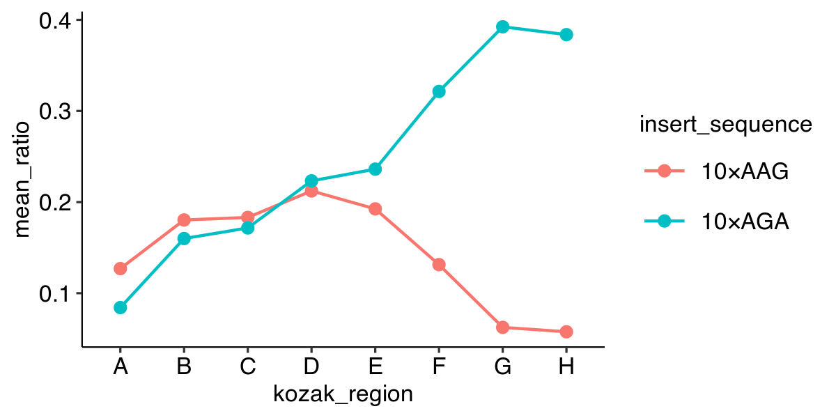
%>% and + if you want to plot
data %>%
  group_by(strain) %>%
  summarize(mean_yfp = mean(yfp), mean_rfp = mean(rfp)) %>%
  mutate(mean_ratio = mean_yfp / mean_rfp) %>%
  left_join(annotations, by = "strain") %>%
  ggplot(aes(x = kozak_region, y = mean_ratio,
             color = insert_sequence, group = insert_sequence)) +
  geom_line() +
  geom_point()
`summarise()` ungrouping output (override with `.groups` argument)