Concepts in Machine Learning Class 2: Supervised Learning
Objectives
Welcome to class 2 of Concepts in Machine Learning!
In the last class, we touched on all of the main concepts that we will be covering in this course including supervised and unsupervised learning, exploratory data analysis, and ethics.
Today we will expand on our knowledge of supervised machine learning. By the end of this class you should be able to:
- Define and understand the limitations of supervised learning
- Differentiate between regression and classification
- Understand basic applications of supervised learning (linear regression, logistic regression)
- Create supervised learning problem statements
Review of last class
Machine learning is:
- A field of study within the larger field of artificial intellegence
- An algorithm that incorporates large datasets into a statistical model and improves with experience
- Especially useful for tackeling problems where you cannot code the rules and that you cannot scale
Machine learning algorithms make use of large datasets. These datasets consist of features, which are measurable metrics that relate to the problem we are trying to solve. Some or all of these features will be used as inputs to create a model that can predict some target output.
- Last class we use the example of predicting whether or not a patient will be diagnosed with cardiovascular disease.
- Age, gender, smoking status, bmi, choelstorol, among other variables were used to predict if a patient will be diagnosed with cardiovascular disease.
- It’s important to remember that these 7-10 features do not capture every factor that might result in someone being diagnosed with cardiovascular disease, but it may capture enough variablity to build a predictive model.
An overview of supervised learning
The goal of supervised machine learning is to fit a model that relates response variables to predictors and can accurately predict the response for future observations of predictor variables. We will cover supervised learning more in depth in class 2 of this series.
Supervised learning is one of the most commonly used forms of machine learning and it’s generally easier to implement and interpret than unsupervised learning alogrithms.
A hallmark of supervised learning algorithms is that they work in two steps: training and testing. This requires training the algorithm on example datasets with inputs that are annotated (or labled) with the correct response. Once training is complete the algorithm will be tested on a seperate labled dataset and it’s performance is evaluated.
Ideally an the algorithm will be specific enough to accurately predict the response variable, but generalizable so that it works with new datasets.
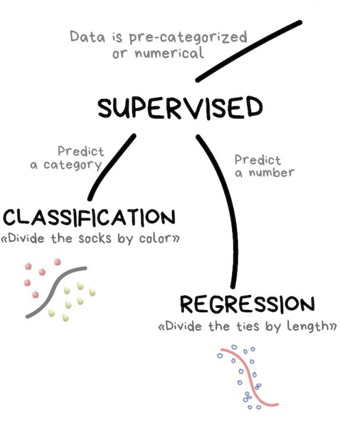
There are two subclasses of supervised learning:
- Regression: predicting a numeric
- Classification: predicting a category
Some basic examples of supervised machine learning
Identifying handwritten letters

- Input: Scanned, handwritten letters
- Output: The actual character
- Dataset: Need thousands of handwritten letters and to annotate the correct letter for each one
Determining if a breast tumor is benign or not from an image

- Input: Images of tumors
- Output: Binary; benign or not
- Dataset: Need a database of medical images, expert diagnosis of benign or not
We will continue to use and expand upon this breast tumor example throughout this class!
How do you train and test a machine?
Training is the hallmark of a supervised learning algorithm because this is the step where a ‘supervisor’ essentially gives the machine the answers. A machine is trained by feeding it large labeled datasets (aka training or validation sets) like we just learned about above. The algorithm works by finding patterns in the dataset and building it’s own set of rules to determine what the outcome might be based on new inputs. When we say large we mean that these training sets should have at a minimum tens of thousands of rows. The more data the better.
Let’s go back to our example of determining if a breast tumor is benign or not from an image. To create an adequate dataset to train on we’d need to collect tens of thousands of images of breast tumors. Then we would need an expert in the field to look at the images and patient medical data to label each image as benign or not. Now that we have labeled images we can train our model. If training is effective our model should be able to accurately predict whether a breast tumor is benign or not when given unlabeled images it’s never seen before.
Testing occurs after you have trained your model. A testing dataset will be similar to the training dataset in that it will have the same features that the algorithm uses to make it’s prediction. The training data must be kept seperate from the data that the algorithm was trained on.
Training a machine starts with data collection
All supervised learning algorithms require large training and testing datasets.
Creating labeled datasets is one of the most time intensive pieces of supervised machine learning. Sometimes this can be done automatically by merging datasets or scraping the internet, but many times the labeling must be done manually. Automatic labelling is quicker and cheaper, but generally messier and less accurate so lots of quality controle and cleaning are required. Manual data collection is expensive and time consuming, but with fewer errors. It’s not uncommon for companies to use their own customers for free labeling. You likely have been involved in some form of labeling yourself!
We will take a more in depth look at what makes a good dataset in class 4 when we discuss exploratory data analysis and ethics.
Data collection and labeling is an intensive process and it can be incredibly difficult to create a comprehensive, ‘good’, dataset. In fact, while some companies might release the source code for their machine learning algorithms, the underlying data that they use is generally kept private because it is so valuable.
Challenge - Data collection
Let’s consider our model for predicting if a breast tumor image is benign or not. What kind of features could we collect from each image to use in our prediction?
Generalization, overfitting, and underfitting
The goal in supervised learning is to build a model that can make accurate prediction on new, unseen datasets that have the same features of the test set used. A model that is capable of making accurate predictions on new data is called generalizable. We want to create a model that can generalize as accurately as possible.
The goal in supervised learning is to build a model that can make accurate prediction on new, unseen datasets that have the same features of the test set used. A model that is capable of making accurate predictions on new data is called generalizable. We want to create a model that can generalize as accurately as possible. Like many of these terms, how generalizable a model is exists on a spectrum. We want our breast tumor predictor to generalize to unseen breast tumor images at a minimum. A best case scenario would be a model that accurately predicts whether or not a tumor is benign with images of tumors from other parts of the body.
If training and testing sets are very similar, we would expect the model to be accurate on the testing set. This might sound like a good thing, however, it can cause problems. We can always build a more and more complex model until we are almost 100 percent accurate on the training set, but the only way to truely test how well a model works on new data is by evaluation on a test set. Simple models will generalize better to new data.
Overfitting occurs when a model is fitted too closely to the specific artifacts of a dataset. In this situation the model will work very well with training data but fail to generalize to new data.
Underfitting occurs when a model is too simple to capture variability in the dataset. In this situation the model won’t work well on the training set.
- Example: “Every tumor with a diameter grater than 10mm is not benign” does not capture any of the variablity in possible outcomes.
Bias-variance trade off
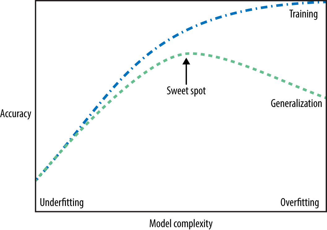
As a model gets more complex, it will become better at predicting on training data. However, if it becomes too complex then it will begin to fail to generalize to new data. This relationship is called the bias-variance trade off.
- Bias is the amount of error introduced by approximating real-world phenomena with a simplified model.
- Variance is how much your model’s test error changes based on variation in the training data. It reflects the model’s sensitivity to the quirks of the dataset it was trained on.
The ideal situation is one where performance is both highly accurate and generalizable to new data. As you can see in the image above on the training set increasing model complexity will result in a more accurate result. However, on the testing set increasing model complexity only works to improve accuracy to an extent after which it become detrimental.
The relationship between model complexity and dataset size
Model complexity is closely tied to the variation of inputs contained in the testing set. Variation can only be comprehensively captured by having very large datasets. You can avoid overfitting by increasing the size of the datasets and therefore increasing the variety of data points in your dataset.
Note!
Adding data points that are duplicates or very similar to those already captured in the dataset will not increase complexity
Two kinds of supervised learning: classification and regression
The main difference between classification and regression is that classification predicts a categorical variable and regression predicts a continuous numerical value.
Classification
Classification aims to predict a class label, which is a choice from a predetermined list of possibilities. When an algorithm is predicting between exactly two class labels we call it binary classification. When an algorithm predicts more than two class labels we call it multiclass classification.
Decision trees and support vector machines are two kinds of classification methods. These methods are different in how they determine which class label to assign. We will focus in on decision trees going forward because they are one of the most simplistic forms of machine learning.
If you’d like to read more about support vector machines check this link out!
Decision trees are a common form of classification
Decision trees are widely used for both classification and regression tasks, but today we will focus on classification with decision trees.
Building a decision tree means the machine is creating the series of if/else questions that will most efficiently lead to the classification decision. Each of these if/else questions is called a ‘test’. The machine learning algorithm iterates over all possible test sequences to find the tree that is most informative and accurate in predicting our target output variable.
You can see how it would be fairly easy to overfit a decision tree. We can keep adding more and more decisions until our training set is perfectly sorted. Two ways to mitigate this with decision trees are:
- Pruning: Removing or collapsing nodes that contain very little information at the bottom of the tree.
- Pre-pruning: Stopping the creation of the tree early by limiting the maximum depth of the tree or requiring a minimum number of data points in a node to keep splitting it.
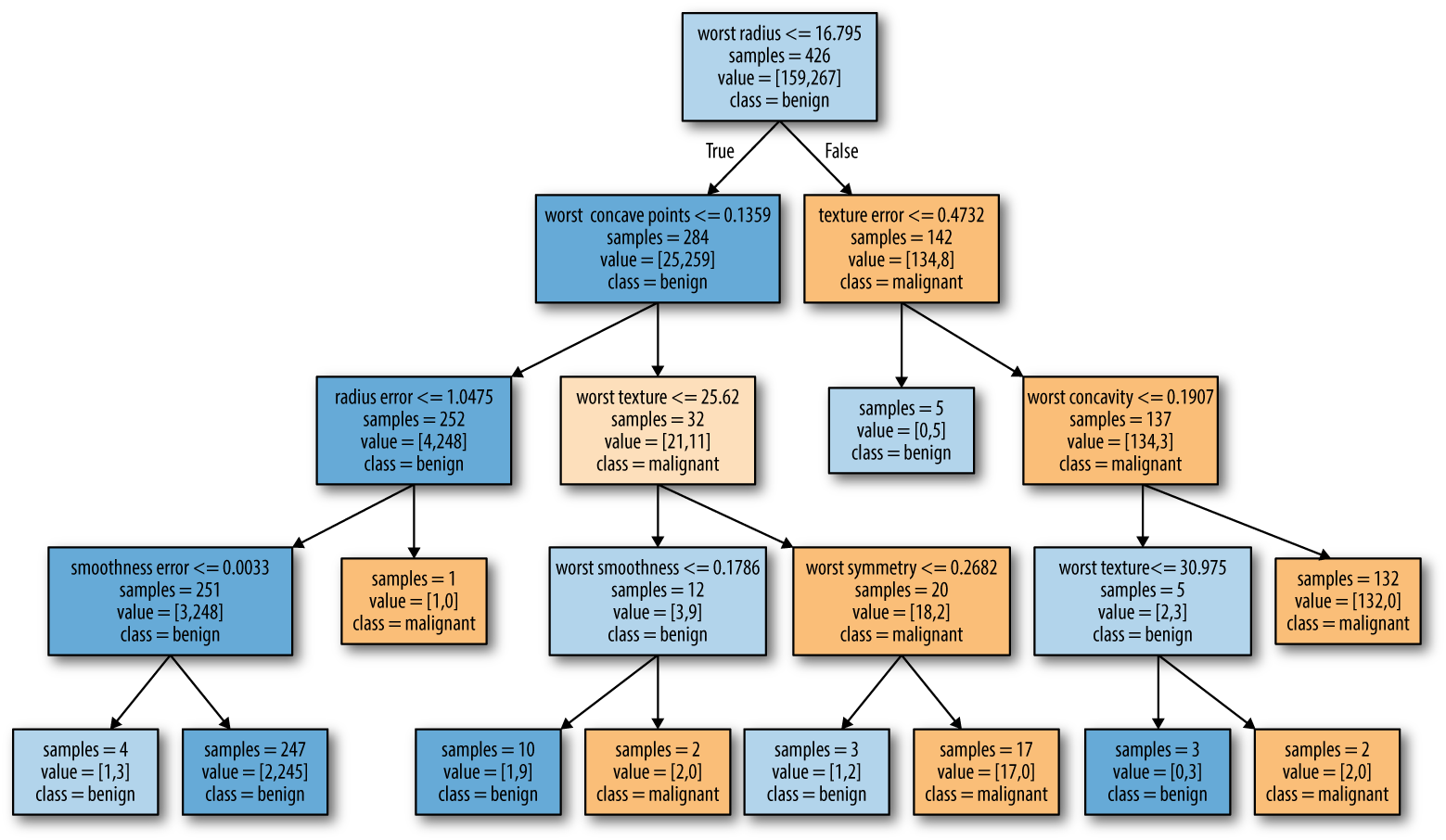
Above is a decision tree built on a breast cancer dataset to predict whether or not a tumor is malignant or benign. This is a relatively small tree with a depth of four and it’s already a bit overwhelming to make sense of. Trees with a depth of ten are not uncommon and are even more difficult to grasp.
It can be helpful to orient yourself by finding out which paths of the tree most data points take. You can assess this on the image above by looking at the samples variable shown in each node.
Feature importance to summarize useful properties in a tree
Feature importance is a method to summarize the inner workings of a decision tree. It captures how important each feature is for the decision the tree makes. It is always a number between 0 and 1, where 0 means a feature wasn’t used at all and 1 means the feature perfectly predicts the target outcome. The feature importance of each feature should always add up to 1.
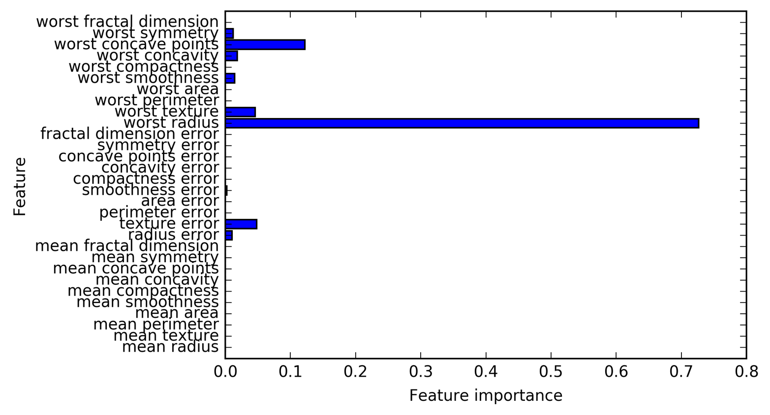
The above image summarizes the feature importance for each feature in the decision tree we discussed previously.
Testing a classification algorithm
A confusion matrix (also known as an error matrix) is a way to test the accuracy of your model. A confusion matrix summerizes the results of the classification algorithm by highlighting false positives, false negatives, true positives, and true negatives.
Below is an example of a confusion matrix for the breast tumor classifier that we have been using as an example.
In this very basic example there are two possible predicted classes: “benign” and “not benign”.
What can we learn from this matrix?
- This classifier made a total of 165 predictions (e.g., 165 breast cancer images were tested).
- Out of those 165 cases, the classifier predicted “benign” 110 times, and “not benign” 55 times.
- In reality, 105 images were of benign tumors, and 60 images were of tumors that are not benign.
Confusion matrix terminology:
- true positives (TP): These are cases in which we predicted benign, and the image is of a benign tumor.
- true negatives (TN): We predicted not benign, and the image is of a tumor that is not benign.
- false positives (FP): We predicted benign, but the image is of a tumor that is not benign. (Also known as a “Type I error.”)
- false negatives (FN): We predicted not benign, but the image is of a tumor that is benign. (Also known as a “Type II error.”)
There are many different metrics that can be derived from a confusion matrix. Two of the most basic metrics are accuracy and the error rate of a classifier.
- Accuracy: A measure of how often the machine guesses correctly
(TP+TN)/total = (100+50)/165 = 0.91
- Error rate: A measure of how often the machine guesses incorrectly
(FP+FN)/total = (10+5)/165 = 0.09- Equivalent to
1 - Accuracy
Note!
This is an example of using a confusion matrix with a binary classifier, but you can easily expand a confusion matrix to evaluate multiclass classifiers.
Regression
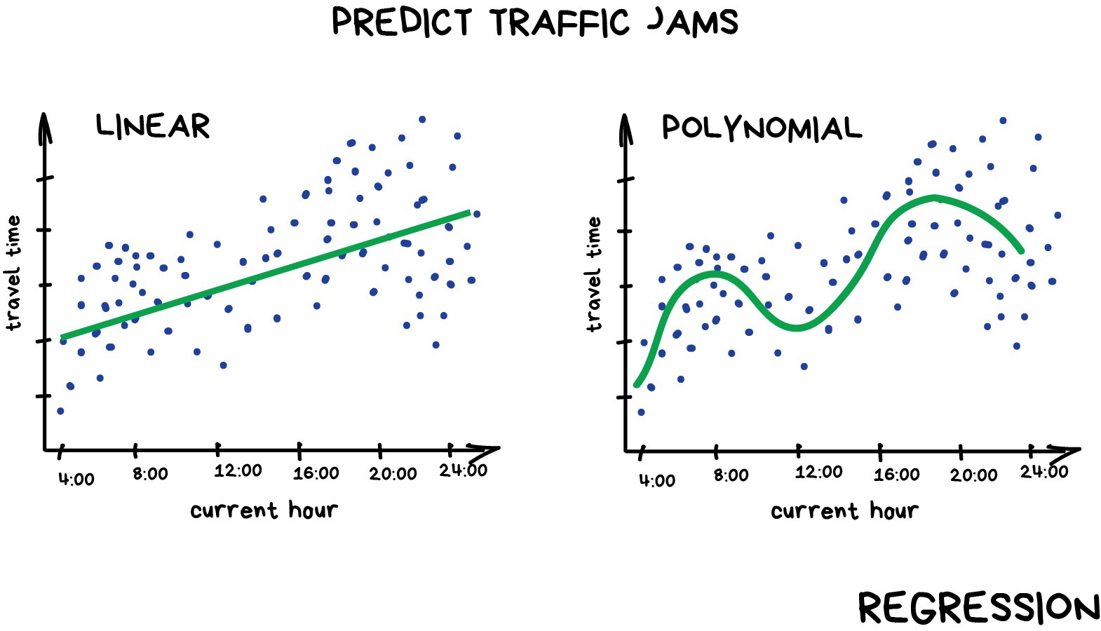
Regression is a form of supervised learning that predicts a continuous numerical value by fitting a line or a curve to the data points. When the algorithm fits a straight line to the data we call this a linear regression. If an algoithm fits a curved line to the data we call it a polynomial regression.
There are different algorithms to fit linear or polynomial lines to data. Ordinary least squares and Ridge regression are two different kinds of regression methods. These methods differ in which metric they use to optimize their best fit line. We will cover ordinary least squares going forward since it is one of the simplest regression methods.
Ordinary least squares (OLS) regression
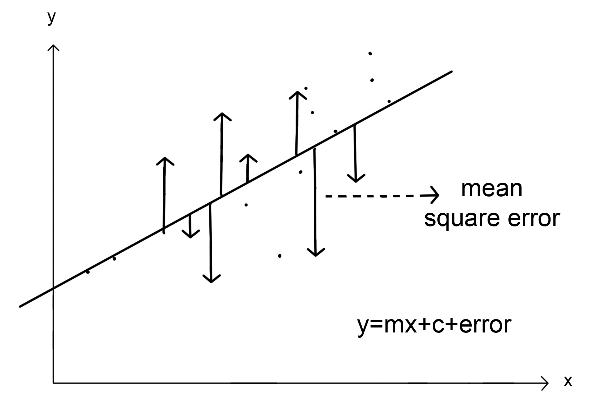
The OLS regression aims to fit a straight line onto the data that minimizes the mean squared error between the predicted value and the true output value. The mean squared error is the sum of the squared differences between the predictions and the true values, divided by the number of samples.
Ordinary least squares regressions, like many other kinds of linear regressions, are very sensitive to outliars!
Testing a regression algorithm
Similarly to classification algorithms, there are many different metrics that can be used when testing and tuning a regression algorithm.
R Squared (R^2) is one of the simplest evaluations of a regression.
- R squared is a very basic indicator of ‘goodness of fit’. It measures how well the regressions predictions approximate the real data points. An R squared of 1 indicates a perfect fit and an R squared of 0 indicates no correlation whatsoever.
Mean squared error (MSE) is another common evaluator
- Here the average squared value of the difference between estimated values and actual values. It measures the quality of the estimator. MSE is always a non-zero number and the closer to zero it is the better the fit.
Some other choices include:
- Root Mean Squared Error (RMSE)
- Mean Absolute Error (MAE)
- Adjusted R Squared (R²)
- Mean Square Percentage Error (MSPE)
- Mean Absolute Percentage Error (MAPE)
- Root Mean Squared Logarithmic Error (RMSLE)
Which metric you will use will be highly dependent the algorithm and context of the analysis.
Wrapping up
Today, we covered some of the main topics of supervised learning. We discussed the importance of data collection, dove into classification methods like decision trees and different kinds of regression methods, and practiced writing supervised learning problem statements. For more in depth information check out the optional materials below. Specifically the Visual intro to Machine Learning has a great visualization of how decision trees work.
Next class we will review concepts from the first two classes and cover unsupervised machine learning methods for clustering and dimensionality reduction.
Extra materials
- An animated, scrolling walkthrough of a decision tree.
- A review of supervised machine learning in population genetics